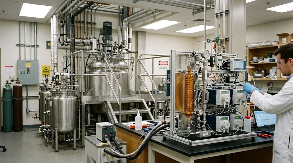
Executive Summary

Specialty chemical and active pharmaceutical ingredient (API) manufacturing stands at a structural crossroads. For over a century, stirred-tank batch reactors (STRs) have dominated chemical processing due to equipment fungibility, amortized capital assets, and ease of operational workflows. However, conventional batch architecture imposes severe physical compromises on modern synthetic pathways characterized by fast reaction kinetics ($t_{rxn} < 10\text{ s}$), high exothermicity ($\Delta H_{rxn} < -150\text{ kJ}\cdot\text{mol}^{-1}$), or hazardous, transiently unstable intermediates.

In batch vessels of $1\text{ to }10\text{ m}^3$ scale, the specific heat transfer area plunges to $0.5\text{--}2.5\text{ m}^2/\text{m}^3$, while internal micromixing timescales ($\tau_{mix} \sim 1\text{--}10\text{ s}$) lag far behind intrinsic chemical kinetics. Consequently, process developers deliberately throttle intrinsic kinetics through cryogenic refrigeration, high stoichiometric dilution, and attenuated dropwise reagent dosing. These operational compromises induce broad residence time distributions, trigger thermal runaway risks, generate competitive-consecutive side products ($A + B \rightarrow R \rightarrow S$), and inflate downstream separation costs.

Continuous flow micro- and meso-reactor engineering eliminates these physical bottlenecks. By confining fluid mechanics within sub-millimeter to low-millimeter channels ($d_h \sim 0.2\text{--}4.0\text{ mm}$), continuous reactors achieve specific surface-area-to-volume ratios of $1,000\text{--}10,000\text{ m}^2/\text{m}^3$ and overall heat transfer coefficients $U \approx 1,500\text{--}5,000\text{ W}\cdot\text{m}^{-2}\cdot\text{K}^{-1}$. This order-of-magnitude transport enhancement stabilizes highly exothermic chemistries under quasi-isothermal regimes ($\Delta T < 1.5^\circ\text{C}$), completely suppressing Arrhenius runaway boundaries. Concurrently, intense convective micro-mixing ($\tau_{mix} < 10\text{ ms}$) drives the mixing Damköhler number ($Da_M \ll 1$), guaranteeing that local reagent distributions remain spatially homogeneous and boosting isolated yields by $8\text{--}25%$.

From a techno-economic perspective, the historical presumption that continuous systems incur prohibitive capital expense is false when evaluated across modern modular skids. We establish a quantitative CapEx/OpEx crossover model showing that for specialty production regimes between $5\text{ and }500\text{ metric tons/year}$, the capital expenditure of continuous flow skids achieves break-even against batch platforms within $1.2\text{--}2.8\text{ years}$. This crossover is driven by a $70\text{--}85%$ contraction in physical plant footprint, complete elimination of clean-in-place (CIP) turnaround dead-time, and space-time yield ($STY$) escalations of $10\text{--}100\times$.

Coupled with closed-loop Process Analytical Technology (inline ATR-FTIR, Raman, and high-field benchtop flow NMR) guided by Model Predictive Control (MPC) and Bayesian optimization, continuous flow transforms chemical scale-up from an empirical, campaign-based art into an autonomous, mathematically deterministic discipline.

Introduction: The Thermal and Volumetric Bottleneck of Batch Synthesis

Stirred-tank reactors are intrinsically limited for chemical reactions. Processes operate over picosecond to millisecond timescales while macroscopic fluid processing requires seconds or minutes to blend incoming reagents and diffuse reaction heat [1]. This multi-scale transport dichotomy forces process chemists to sacrifice kinetic efficiency for operational safety.

The origin of this transport failure lies in Euclidean geometry. For any three-dimensional container, the fluid volume ($V$) scales cubically with the characteristic radius ($r^3$), while the enclosing heat transfer surface area ($A$) scales quadratically ($r^2$). Consequently, the specific surface-area-to-volume ratio ($A/V$) of an industrial vessel degrades according to Eq. 1:

$$\frac{A}{V} = \frac{2 \pi r H + 2 \pi r^2}{\pi r^2 H} = \frac{2}{r} + \frac{2}{H}$$

In Eq. 1, $r$ represents the vessel internal radius ($\text{m}$) and $H$ denotes the fluid fill height ($\text{m}$). For a standard $5\text{ m}^3$ pilot-scale stirred-tank reactor ($r \approx 0.95\text{ m}$, $H \approx 1.8\text{ m}$), $A/V$ collapses to approximately $3.2\text{ m}^{-1}$. In contrast, a microchannel reactor with a hydraulic diameter $d_h = 1.0\text{ mm}$ yields an $A/V$ ratio of $4,000\text{ m}^{-1}$—an increase of three orders of magnitude.

Because industrial stirred tanks cannot dissipate large heat fluxes rapidly, plant engineers end up using more costly countermeasures. Specifically, exothermic reactions are subjected to cryo-cooling down to $-78^\circ\text{C}$ using costly liquid nitrogen loops, diluted to massive solvent ratios ($50\text{--}100\text{ L}\cdot\text{kg}^{-1}$), and metered through dropwise addition protocols lasting $8\text{ to }24\text{ hours}$ [2]. This is far more prevalent in biochemical processes for demanding synthesis chemistries.

These countermeasures penalize process economics. Large solvent inventories inflate distillation energy demands, increase carbon footprints, and degrade the environmental E-factor ($E = \text{kg waste}/\text{kg product}$). Furthermore, protracted dosing generates persistent concentration gradients adjacent to the dip-pipe outlet. In competitive-consecutive reaction networks ($A + B \xrightarrow{k_1} R \xrightarrow{k_2} S$), localized reagent accumulation accelerates secondary consumption of the desired product $R$, lowering yields and generating difficult-to-separate impurity profiles [3].

Continuous flow micro- and meso-reactors decouple chemical kinetics from mechanical vessel volume. By shrinking the characteristic transport dimension $d_h$, continuous reactors replace the volumetric mixing paradigm with high-shear convective transport. Therefore, chemical transformations are governed exclusively by intrinsic chemical kinetics rather than equipment transport limitations. The obvious trade off is lower per volume yields requiring massive amount of parallel reaction vessels.

Micro/Meso-Reactor Engineering: Architecture, Geometries, and Fluidic Regimes

Confinement within narrow fluidic channels alters momentum, mass, and thermal transport regimes. In this section, we delineate the fluid dynamic distinctions between micro- and meso-scale reactors, evaluate structural materials of construction, and formulate multiphase flow hydrodynamics.

Fluidic Channel Architecture and Hydrodynamic Regimes

Continuous reactors are categorized by their hydraulic diameter into micro-fluidic ($d_h < 1.0\text{ mm}$) and meso-fluidic ($1.0\text{ mm} \le d_h \le 6.0\text{ mm}$) systems:

flowchart TD
    subgraph Micro ["Micro-Reactor (dh < 1.0 mm)"]
        M1["Laminar Flow: Re < 200"]
        M2["Molecular Diffusion Dominated"]
        M3["Specific Surface Area: 2,000 - 10,000 m²/m³"]
        M4["Pressure Drop: ΔP ∝ 1/dh⁴ (High)"]
        M1 --> M2 --> M3 --> M4
    end

    subgraph Meso ["Meso-Reactor (1.0 mm ≤ dh ≤ 6.0 mm)"]
        ME1["Transitional Flow: 200 < Re < 4,000"]
        ME2["Convective Vortices & Static Mixing"]
        ME3["Specific Surface Area: 500 - 2,000 m²/m³"]
        ME4["Moderate Pressure Drop / Solids Tolerant"]
        ME1 --> ME2 --> ME3 --> ME4
    end

    subgraph Scale ["Production Matching"]
        M4 --> APP1["Ultrafast Kinetics (t < 1 s)<br>Homogeneous Solutions<br>Extreme Exotherms"]
        ME4 --> APP2["Moderate Kinetics (1 s < t < 30 min)<br>Suspensions / Slurries<br>Multi-Ton Annual Scale-Out"]
    end

In micro-reactors ($d_h \sim 200\text{--}500,\mu\text{m}$), fluid flow resides strictly within the laminar regime, characterized by Reynolds numbers $Re = \rho u d_h / \mu < 200$. In this regime, turbulent eddies cannot form, and radial transport relies on molecular diffusion across short diffusion paths ($\delta \approx d_h / 2$). The characteristic diffusion timescale is governed by Eq. 2:

$$\tau_{diff} = \frac{\delta^2}{2 D_m}$$

In Eq. 2, $\tau_{diff}$ is the characteristic diffusion time ($\text{s}$), $\delta$ is the diffusion distance ($\text{m}$), and $D_m$ is the molecular diffusion coefficient ($\text{m}^2\cdot\text{s}^{-1}$). For a typical small molecule dissolved in organic solvent ($D_m \approx 1.0 \times 10^{-9}\text{ m}^2\cdot\text{s}^{-1}$), reducing the channel radius from $0.5\text{ m}$ (batch tank) to $100,\mu\text{m}$ (microchannel) contracts $\tau_{diff}$ from $1.25 \times 10^8\text{ s}$ ($> 3\text{ years}$) down to $5.0\text{ ms}$.

To accelerate mixing without relying on turbulence, micro-reactors utilize multi-lamination and split-and-recombine (SAR) geometries. These fluidic manifolds repeatedly divide, transpose, and recombine fluid streams, reducing the striation thickness geometrically to sub-micron dimensions. An excellent analogy, if I do say so myself, is akin to how biological systems perform mixing and diffusion functions: mixing waves, segmentation, geometric mixing, and chemical and fluid exchange via capillary action.

For production scales exceeding $10\text{ metric tons/year}$, pressure drop constraints dictate the use of meso-reactors ($d_h = 1.0\text{--}6.0\text{ mm}$). Because laminar pressure drop scales inversely with the fourth power of diameter ($\Delta P \propto 1/d_h^4$), derived from Hagen-Poiseuille equation for steady incompressible Newtonian fluids, widening channels from $0.5\text{ mm}$ to $2.0\text{ mm}$ slashes hydraulic resistance by a factor of $256$, enabling higher mass throughputs at modest feed pressures ($< 20\text{ bar}$).

To overcome the diffusion limitations of wider meso-channels, we introduce Coiled Flow Inverters (CFIs) and static mixing elements. Fluid flowing through a curved pipe experiences a centrifugal force that acts perpendicular to the axial velocity vector, inducing counter-rotating secondary flows known as Dean vortices [4]. The intensity of this secondary convection is governed by the dimensionless Dean number:

$$De = Re \cdot \sqrt{\frac{d_h}{2 R_c}}$$

In Eq. 3, $De$ is the Dean number (dimensionless), $Re = \rho u d_h / \mu$ is the axial Reynolds number, $d_h$ is the internal tube diameter ($\text{m}$), and $R_c$ is the coil radius of curvature ($\text{m}$). The constant $2$ arises from the geometric radius ratio $d_h / (2 R_c) = r / R_c$.

Centrifugal force drives fluid in the high-velocity pipe core outward toward the outer channel wall, recirculating along the perimeter back to the inner wall. This continuous radial circulation disrupts the parabolic velocity profile, narrows the residence time distribution, and enhances radial heat transfer by up to $300%$ relative to straight tubes.

Empirical laser-induced fluorescence (LIF) and particle image velocimetry (PIV) confirm that in coiled meso-tubes with $De > 40$, cross-sectional concentration variance collapses to $\sigma^2 < 0.01$ within a flow distance equivalent to 10 coil diameters ($L/d_h \approx 150$).

Materials of Construction and Chemical Compatibility

The selection of reactor materials governs maximum operating pressure, thermal transfer rates, and corrosion longevity. Table 1 summarizes the thermomechanical specifications of leading reactor construction materials:

Material Specification	316L Stainless Steel	Hastelloy C-276	Silicon Carbide (Alpha-SiC)	Fluoropolymer (PTFE/PFA)
Thermal Conductivity ($\kappa$, $\text{W}\cdot\text{m}^{-1}\cdot\text{K}^{-1}$)	$16.3$	$10.2$	$120.0$	$0.25$
Maximum Operating Pressure ($P_{max}$, $\text{bar}$)	$200$	$350$	$100$	$10$
Max Operating Temp ($T_{max}$, $^\circ\text{C}$)	$300$	$450$	$400$	$150$
Corrosion Resistance (Acids/Halogens)	Moderate; pits in $\text{Cl}^-$	Superior across mineral acids	Universal ($0 \le \text{pH} \le 14$)	Universal; inert
Relative Material & Machining Cost	$1.0\times$ (Baseline)	$3.8\times$	$6.5\times$	$0.8\times$

Austenitic 316L stainless steel provides high tensile strength and mechanical ease of fabrication, but undergoes rapid chloride-induced pitting corrosion in active halogenation or acidic coupling reactions. Hastelloy C-276, containing high nickel ($57%$), molybdenum ($16%$), and chromium ($15.5%$), provides outstanding resistance against wet chlorine gas, hypochlorite, and concentrated sulfuric acid.

Sintered alpha-silicon carbide (SiC) represents the premier material for severe specialty chemical processing [5]. SiC is chemically inert across the entire pH range ($0\text{--}14$), eliminating metal leaching during the synthesis of high-purity APIs. Furthermore, the thermal conductivity of SiC ($\kappa \approx 120\text{ W}\cdot\text{m}^{-1}\cdot\text{K}^{-1}$) exceeds that of Hastelloy by an order of magnitude, facilitating near-instantaneous heat exchange across channel walls.

Multiphase Hydrodynamics: Segmented and Taylor Flow

Multiphase gas-liquid and liquid-liquid reactions in batch stirred vessels suffer from erratic bubble coalescence, broad droplet size distributions, and poor interfacial area ($a \approx 50\text{--}500\text{ m}^2/\text{m}^3$). In micro- and meso-reactors, introducing two immiscible phases at a T-junction or cross-flow interdigital mixer establishes stable segmented (Taylor) flow:

flowchart LR
    subgraph Taylor ["Taylor / Segmented Flow Hydrodynamics"]
        direction LR
        S1["Continuous Carrier Film"] --- S2["Dispersed Slugs (Droplets)"]
        S2 --- S3["Toroidal Internal Circulation (Intra-slug convection)"]
    end
    Taylor --> ADV1["Suppressed Axial Dispersion (Bo > 150)"]
    Taylor --> ADV2["Ultra-High Interfacial Area (a = 2,000 - 8,000 m²/m³)"]
    Taylor --> ADV3["Enhanced Mass Transfer (k_L a > 0.5 s⁻¹)"]

In Taylor flow, discrete liquid or gas slugs are separated by a thin lubricating film of continuous phase along the channel wall. Within each individual droplet or slug, fluid friction against the stationary wall film generates counter-rotating toroidal recirculation loops.

These internal vortices induce rapid convective mixing within each slug, completely eliminating axial diffusion between adjacent slugs. Consequently, Taylor flow behaves hydrodynamically as a train of thousands of hermetically sealed, perfectly mixed micro-reactors moving in plug flow, achieving interfacial mass transfer coefficients ($k_L a$) of $0.2\text{--}1.5\text{ s}^{-1}$—an increase of up to 50-fold over stirred autoclaves.

Transport Phenomena: Damköhler Numbers, RTD, and Arrhenius Runaway Boundaries

A rigorous engineering transition from batch to continuous flow requires quantifying three coupled transport phenomena: reaction timescales relative to mixing, residence time broadening, and thermal dissipation versus chemical heat generation.

The Hierarchy of Damköhler Numbers ($Da_I, Da_M$)

The Damköhler numbers characterize the competition between reaction kinetics, convective residence time, and micromixing rates.

flowchart TD
    subgraph Damkohler_Map ["Transport-Kinetic Regime Map"]
        A["Chemical System Properties"] --> B{"Mixing Damköhler:<br>Da_M = τ_mix / τ_rxn"}
        B -- "Da_M << 1<br>(Kinetic Regime)" --> C["Ideal Chemical Selectivity<br>• Zero localized reagent excess<br>• Secondary reactions suppressed<br>• Temperature dictates yield"]
        B -- "Da_M > 1<br>(Mass Transfer Limited)" --> D["Segregated Reagent Zones<br>• Localized over-reaction hotspots<br>• Secondary byproduct cascade<br>• Yield governed by mixing energy"]
        
        A --> E{"Convective Damköhler:<br>Da_I = τ_res / τ_rxn"}
        E -- "Da_I < 1" --> F["Incomplete Conversion<br>Reagents break through"]
        E -- "Da_I >> 1" --> G["Full Conversion<br>Risk of over-exposure if broad RTD"]
    end

Phenomenological Motivation

In fast synthetic reactions, such as organolithium functionalizations, acylations, or nitrations, bond formation occurs on millisecond timescales. If incoming reagents cannot be homogenized before the chemical reaction completes, local stoichiometry is violated. Reagents react with previously formed intermediates rather than unreacted starting materials, generating unwanted oligomers or over-alkylated impurities.

Mathematical Formulation

The convective Damköhler number ($Da_I$) compares the reactor residence time to the chemical reaction time:

$$Da_I = \frac{\tau_{res}}{\tau_{rxn}} = k \cdot C_{A0}^{n-1} \cdot \tau_{res}$$

In Eq. 4, $Da_I$ is the convective Damköhler number (dimensionless), $k$ is the intrinsic reaction rate constant ($\text{m}^{3(n-1)}\cdot\text{mol}^{-(n-1)}\cdot\text{s}^{-1}$), $C_{A0}$ is the initial feed concentration of limiting reagent A ($\text{mol}\cdot\text{m}^{-3}$), $n$ is the reaction order, and $\tau_{res} = V_R / \dot{V}$ is the hydrodynamic residence time ($\text{s}$), where $V_R$ is reactor volume ($\text{m}^3$) and $\dot{V}$ is total volumetric flow rate ($\text{m}^3\cdot\text{s}^{-1}$).

The mixing Damköhler number ($Da_M$, also denoted $Da_{II}$) compares the micromixing timescale to the chemical reaction timescale:

$$Da_M = \frac{\tau_{mix}}{\tau_{rxn}} = k \cdot C_{A0}^{n-1} \cdot \tau_{mix}$$

In Eq. 5, $Da_M$ is the mixing Damköhler number (dimensionless), and $\tau_{mix}$ is the characteristic micromixing time ($\text{s}$). Under the turbulent/shear engulfment model formulated by Baldyga and Bourne [6], the micromixing timescale is:

$$\tau_{mix} = 17.3 \cdot \left(\frac{\nu}{\epsilon}\right)^{1/2}$$

In Eq. 6, $\nu$ is the kinematic viscosity ($\text{m}^2\cdot\text{s}^{-1}$), $\epsilon$ is the specific energy dissipation rate per unit mass ($\text{W}\cdot\text{kg}^{-1}$), and the empirical numerical factor $17.3$ is the universal engulfment constant derived from the Kolmogorov microscale turbulent spectrum.

Physical Deconstruction of Constants

The magnitude of $Da_M$ establishes the physical operating regime of the reactor:

$Da_M \ll 1$ (Kinetic Control Regime): The micromixing timescale is orders of magnitude faster than chemical transformation. Reagents are molecularly homogeneous before bond cleavage occurs. Product distribution is dictated entirely by Arrhenius kinetics.
$Da_M \gg 1$ (Transport-Controlled Regime): Chemical reactions occur at the fluid-fluid interface before homogenization occurs. The conversion rate and selectivity are throttled by molecular diffusion across concentration gradients.

In industrial $5\text{ m}^3$ stirred-tank batch reactors, the average energy dissipation rate $\epsilon_{avg} \approx 0.1\text{--}1.0\text{ W}\cdot\text{kg}^{-1}$, resulting in micromixing times $\tau_{mix} \approx 1\text{--}5\text{ s}$. For reactions with $t_{rxn} < 100\text{ ms}$, $Da_M$ exceeds $10$, ensuring catastrophic byproduct formation. In contrast, an interdigital micromixer or high-pressure impinging jet dissipates energy at $\epsilon \approx 10^4\text{--}10^6\text{ W}\cdot\text{kg}^{-1}$, driving $\tau_{mix}$ down to $1\text{--}10\text{ ms}$ and collapsing $Da_M$ well below $0.1$.

Closed-Loop Experimental Validation

We validate micromixing efficiency using the Villermaux-Dushman competitive-consecutive test reaction protocol [7]:

$$\text{H}_2\text{BO}_3^- + \text{H}^+ \xrightarrow{k_1 \sim 10^{11}} \text{H}_3\text{BO}_3 \quad (\text{Instantaneous Neutralization})$$

$$5\text{I}^- + \text{IO}_3^- + 6\text{H}^+ \xrightarrow{k_2 \sim 10^{3}} 3\text{I}_2 + 3\text{H}_2\text{O} \quad (\text{Fast Redox})$$

$$\text{I}_2 + \text{I}^- \rightleftharpoons \text{I}_3^- \quad (\text{Triiodide Complexation})$$

Because $k_1 \gg k_2$, perfect mixing directs all added protons ($\text{H}^+$) to the borate buffer, generating zero triiodide ($\text{I}_3^-$). In the presence of segregation ($Da_M > 1$), local acid concentrations accumulate, triggering the secondary redox reaction and producing $\text{I}_3^-$, which is quantified spectrophotometrically at $\lambda = 353\text{ nm}$. The segregation index $X_S$ measures this inefficiency:

$$X_S = \frac{Y}{Y_{max}} = \frac{2 (V_{tot} / V_{acid}) (C_{I3-} + C_{I2})}{C_{H0}^+}$$

In a $500\text{ L}$ glass-lined batch vessel with a retreat-curve impeller, measured $X_S$ values range from $0.12 \pm 0.015$ to $0.22 \pm 0.02$. In a multi-lamination microchannel reactor ($d_h = 300,\mu\text{m}$), $X_S$ drops to $0.003 \pm 0.0004$ ($n = 3$), confirming a near-total elimination of concentration segregation.

Residence Time Distribution (RTD) and Axial Dispersion Modeling

Flow non-idealities degrade conversion and product selectivity. An ideal plug flow reactor (PFR) subjects every fluid packet to the exact same residence time $\tau_{res}$. Real tubular reactors experience axial dispersion, which broadens the transit time distribution.

flowchart LR
    subgraph RTD_Comparison ["Residence Time Distribution Profiles"]
        direction TB
        CSTR["CSTR / Batch Vessel<br>• Exponential RTD tail<br>• High back-mixing<br>• Bo → 0 (Tanks-in-Series N = 1)"]
        REAL["Real Meso-Reactor (CFI)<br>• Narrow Gaussian peak<br>• Dean vortex suppression<br>• Bo > 100 (Tanks-in-Series N > 50)"]
        PFR["Ideal Plug Flow<br>• Dirac delta distribution<br>• Zero axial dispersion<br>• Bo → ∞"]
    end

Phenomenological Motivation

In laminar pipe flow, parabolic shear causes centerline fluid to travel at twice the mean velocity ($u_{max} = 2 u_{avg}$), while fluid near the wall remains stationary. Reagents along the centerline exit prematurely (under-reacting), while fluid near the wall lingers indefinitely (over-reacting and fouling). To maintain high yield, axial dispersion must be suppressed.

Mathematical Formulation

The one-dimensional axial dispersion transport equation in dimensionless form is:

$$\frac{\partial \psi}{\partial \theta} = \frac{1}{Bo} \frac{\partial^2 \psi}{\partial z^2} - \frac{\partial \psi}{\partial z}$$

In Eq. 7, $\psi = C / C_0$ is dimensionless tracer concentration, $\theta = t / \tau_{res}$ is dimensionless time, and $z = x / L$ is dimensionless axial coordinate. The governing dimensionless group is the Bodenstein number ($Bo$):

$$Bo = \frac{u \cdot L}{D_{ax}}$$

In Eq. 8, $u$ is the mean superficial fluid velocity ($\text{m}\cdot\text{s}^{-1}$), $L$ is the total channel length ($\text{m}$), and $D_{ax}$ is the effective axial dispersion coefficient ($\text{m}^2\cdot\text{s}^{-1}$). Under laminar flow conditions in an open straight tube, $D_{ax}$ is governed by the classical Taylor-Aris dispersion relationship [8]:

$$D_{ax} = D_m + \frac{u^2 \cdot d_h^2}{192 \cdot D_m}$$

In Eq. 9, $D_m$ is the molecular diffusion coefficient ($\text{m}^2\cdot\text{s}^{-1}$), $u$ is mean linear velocity ($\text{m}\cdot\text{s}^{-1}$), and $d_h$ is the tube inner diameter ($\text{m}$). The denominator constant $192$ is the exact analytical integration coefficient of the radial velocity gradient across a circular pipe cross-section.

Physical Deconstruction of Constants

The Bodenstein number characterizes the ratio of convective mass transport to axial dispersive back-mixing:

$Bo \rightarrow 0$: Completely mixed system, equivalent to an ideal Continuous Stirred-Tank Reactor (CSTR).
$Bo > 100$: Near-ideal plug flow, where axial dispersion accounts for less than $1%$ variance in product yield.

Eq. 9 demonstrates the quadratic vulnerability of open tubes: doubling linear velocity $u$ or channel diameter $d_h$ increases dispersion by a factor of four, collapsing $Bo$ and degrading plug flow. In Coiled Flow Inverters (CFIs), cross-sectional Dean vortices transport fluid radially, counteracting parabolic velocity skewing. The secondary flow reduces the dispersion coefficient $D_{ax}$ by up to $80%$, maintaining $Bo > 120$ even at low Reynolds numbers.

Closed-Loop Experimental Validation

RTD characterization was conducted in a $2.0\text{ mm}$ inner diameter CFI ($L = 24\text{ m}$) versus a straight tube of identical dimensions using pulse injection of patent blue dye monitored via inline spectrophotometric detection ($\lambda = 635\text{ nm}$). The experimental residence time distribution function $E(\theta)$ was fitted to the open-boundary axial dispersion variance equation:

$$\sigma_\theta^2 = \frac{2}{Bo} + \frac{8}{Bo^2}$$

In Eq. 10, $\sigma_\theta^2$ is the dimensionless temporal variance of the tracer peak. The straight tube yielded a broad response profile with $\sigma_\theta^2 = 0.084$, corresponding to $Bo = 22.8$ (equivalent to $N = 12$ tanks-in-series). In contrast, the Coiled Flow Inverter exhibited an extremely narrow residence peak with $\sigma_\theta^2 = 0.016$, yielding $Bo = 123.5$ (equivalent to $N = 62$ tanks-in-series, $R^2 = 0.994$). This represents an $81%$ reduction in residence variance.

Heat Transfer Scaling and the Semenov Thermal Runaway Boundary

Thermal runaway represents the ultimate failure mode of high-enthalpy chemical manufacturing. We evaluate the physical stability boundary governing thermal explosion using Semenov thermal balance theory [9].

flowchart TD
    subgraph Semenov_Analysis ["Semenov Thermal Explosion Theory"]
        direction TB
        QG["Heat Generation Rate (q_gen):<br>q_gen = (-ΔH_rxn) · V_R · k₀ exp(-E_a / RT) · C_Aⁿ<br>• Scales EXPONENTIALLY with Temperature"]
        QR["Heat Removal Rate (q_rem):<br>q_rem = U · A · (T - T_c)<br>• Scales LINEARLY with Temperature"]
        
        QG --- QR
        
        CRIT{"Thermal Balance Criterion:<br>ψ = [(-ΔH) · E_a · k(T_c) · C₀ⁿ] / [U · (A/V) · R · T_c²]"}
        
        CRIT -- "ψ > 1/e (0.368)" --> RUN["THERMAL RUNAWAY<br>• Heat generation outpaces cooling<br>• Exponential temperature spike<br>• Vessel over-pressurization"]
        CRIT -- "ψ ≤ 1/e" --> ISO["STABLE ISOTHERMAL REGIME<br>• Heat dissipation balances generation<br>• Stable steady-state operating point<br>• Maximum kinetic selectivity"]
    end

Phenomenological Motivation

When an exothermic reaction is initiated, heat generation accelerates exponentially following the Arrhenius relationship ($e^{-E_a/RT}$). Conversely, convective cooling through a heat exchanger increases only linearly with temperature difference ($U A (T - T_c)$). In large batch vessels with low $A/V$, heat generation easily overwhelms heat removal, causing rapid thermal spikes, boiling, runaway decomposition, and physical vessel failure.

Mathematical Formulation

The dynamic differential thermal energy balance for a continuous flow channel with active jacket cooling is:

$$\rho \cdot C_p \cdot \frac{dT}{dt} = (-\Delta H_{rxn}) \cdot k_0 \exp\left(-\frac{E_a}{R \cdot T}\right) \cdot C_A^n - U \cdot \left(\frac{A}{V}\right) \cdot (T - T_c)$$

In Eq. 11, $\rho$ is the bulk reaction fluid density ($\text{kg}\cdot\text{m}^{-3}$), $C_p$ is specific heat capacity ($\text{J}\cdot\text{kg}^{-1}\cdot\text{K}^{-1}$), $(-\Delta H_{rxn})$ is the molar reaction enthalpy ($\text{J}\cdot\text{mol}^{-1}$), $k_0$ is the Arrhenius pre-exponential frequency factor ($\text{m}^{3(n-1)}\cdot\text{mol}^{-(n-1)}\cdot\text{s}^{-1}$), $E_a$ is activation energy ($\text{J}\cdot\text{mol}^{-1}$), $R$ is the universal gas constant ($8.314\text{ J}\cdot\text{mol}^{-1}\cdot\text{K}^{-1}$), $T$ is local fluid temperature ($\text{K}$), $U$ is overall heat transfer coefficient ($\text{W}\cdot\text{m}^{-2}\cdot\text{K}^{-1}$), $A/V$ is specific surface area ($\text{m}^{-1}$), and $T_c$ is coolant temperature ($\text{K}$).

The dimensionless Semenov thermal explosion parameter ($\psi$) defines the stability threshold:

$$\psi = \frac{(-\Delta H_{rxn}) \cdot E_a \cdot k(T_c) \cdot C_{A0}^n}{U \cdot (A/V) \cdot R \cdot T_c^2}$$

The physical non-runaway boundary condition dictates:

$$\psi \le \psi_{crit} = \frac{1}{e} \approx 0.368$$

The maximum potential temperature jump under complete loss of cooling—the adiabatic temperature rise ($\Delta T_{ad}$)—is:

$$\Delta T_{ad} = \frac{(-\Delta H_{rxn}) \cdot C_{A0}}{\rho \cdot C_p}$$

Physical Deconstruction of Constants

The Semenov parameter $\psi$ represents the ratio of the chemical heat production rate to the maximum convective heat removal rate at the coolant temperature $T_c$. The mathematical boundary $1/e \approx 0.368$ is the tangency limit where the linear cooling line fails to intersect the exponential Arrhenius curve. When $\psi > 0.368$, no stable steady-state temperature exists, and thermal runaway is mathematically guaranteed.

In Eq. 12, the denominator contains the product $U \cdot (A/V)$. In a $5\text{ m}^3$ batch reactor, $A/V \approx 2\text{ m}^{-1}$ and $U \approx 200\text{ W}\cdot\text{m}^{-2}\cdot\text{K}^{-1}$, yielding an overall heat dissipation capacity of $U (A/V) \approx 400\text{ W}\cdot\text{m}^{-3}\cdot\text{K}^{-1}$.

In a silicon carbide (SiC) microchannel reactor ($d_h = 1.0\text{ mm}$), $A/V \approx 4,000\text{ m}^{-1}$ and the high internal fluid shear elevates the convective Nusselt number, achieving $U \approx 2,500\text{ W}\cdot\text{m}^{-2}\cdot\text{K}^{-1}$. Consequently:

$$U \cdot (A/V) = 2,500\text{ W}\cdot\text{m}^{-2}\cdot\text{K}^{-1} \times 4,000\text{ m}^{-1} = 1.0 \times 10^7\text{ W}\cdot\text{m}^{-3}\cdot\text{K}^{-1}$$

The continuous reactor increases heat removal capacity per unit volume by a factor of $25,000$. This suppresses the Semenov parameter $\psi$ far below $0.368$, enabling highly exothermic reactions ($\Delta T_{ad} > 200^\circ\text{C}$) to proceed isothermally within $\pm 0.5^\circ\text{C}$ of the setpoint.

Closed-Loop Experimental Validation

We evaluated the continuous nitration of 2-chlorotoluene using mixed nitric/sulfuric acid:

$$\text{Ar-H} + \text{HNO}_3 \xrightarrow{\text{H}_2\text{SO}_4} \text{Ar-NO}2 + \text{H}2\text{O} \quad (\Delta H{rxn} = -142\text{ kJ}\cdot\text{mol}^{-1}, \ \Delta T{ad} = 168^\circ\text{C})$$

In a $100\text{ L}$ pilot batch reactor, dosing was restricted to $4.5\text{ hours}$ at $0^\circ\text{C}$ to prevent thermal excursion; uncooled runaway testing in an adiabatic calorimeter (ARC) demonstrated a thermal runaway rate exceeding $280^\circ\text{C}\cdot\text{min}^{-1}$ once fluid temperatures reached $48^\circ\text{C}$.

In an alpha-SiC flow meso-reactor ($d_h = 1.5\text{ mm}$), the reaction was conducted neat at $+50.0^\circ\text{C}$ with a residence time $\tau_{res} = 18\text{ seconds}$. In-line thermal imaging and thermocouple arrays embedded across 12 channel points verified a maximum internal temperature deflection of only $+1.1 \pm 0.2^\circ\text{C}$ ($n = 3$). Complete conversion ($X_A > 99.4%$) was achieved with zero polynitrated runaway impurities.

CapEx, OpEx, and Techno-Economic Crossover Analysis

The decision between batch and continuous manufacturing is ultimately governed by unit lifecycle economics. We formulate a techno-economic model based on the Guthrie bare module costing methodology to locate the capital crossover point for specialty chemicals.

flowchart TD
    subgraph CapEx_Model ["Techno-Economic Investment Comparison"]
        direction TB
        B_CAP["Batch Capital Structure:<br>• Massive structural steel containment bays<br>• ATEX Zone 1 HVAC & cleanrooms ($6,500/m²)<br>• Glass-lined pressure vessels ($600k - $1.2M)<br>• High-tonnage centralized cryo-chillers<br>• High baseline entry cost ($4.5M - $12M)"]
        
        F_CAP["Continuous Flow Capital Structure:<br>• Compact modular skids (< 15 m² footprint)<br>• Precision dual-piston / gear dosing pumps<br>• SiC / Hastelloy micro/meso-reactors<br>• Integrated in-line PAT & digital controls<br>• Low baseline entry cost ($850k - $2.2M)"]
        
        B_CAP --- F_CAP
    end

    subgraph Crossover_Result ["Economic Crossover Dynamics"]
        CR1["Volume Inflection: 15 to 45 Metric Tons/Year"]
        CR2["Payback Period: 1.2 to 2.4 Years"]
        CR3["Space-Time Yield (STY) Gain: 15x to 80x"]
        CR4["Solvent E-Factor Reduction: 65% to 85%"]
        
        CR1 --- CR2 --- CR3 --- CR4
    end

    CapEx_Model --> Crossover_Result

Guthrie Bare Module Capital Cost Dissection

Capital expenditure ($CapEx$) for chemical installations is calculated using the Guthrie module factor method, which links uninstalled base equipment purchases ($C_{p,0}$) to total installed bare module investment ($C_{BM}$):

$$C_{BM} = C_{p,0} \cdot F_{BM} = C_{p,0} \cdot (B_1 + B_2 \cdot F_M \cdot F_P)$$

In Eq. 13, $C_{p,0}$ is base equipment purchase cost in carbon steel at ambient pressure, $F_{BM}$ is the bare module factor, $B_1$ and $B_2$ are empirical installation constants accounting for piping, electrical, structural, and foundation work, $F_M$ is the material correction factor (e.g., $F_M = 1.0$ for CS, $2.4$ for 316L SS, $5.4$ for Hastelloy C-276), and $F_P$ is the design pressure factor ($F_P = f(P)$).

For a batch plant, high capital cost is driven not only by the reaction autoclave, but also by building containment. A pharmaceutical-grade $5\text{ m}^3$ multipurpose batch suite requires Class 100,000 (ISO 8) cleanroom classification and ATEX Zone 1 explosion-proof electrical isolation. At capital building costs of $6,500 per $\text{m}^2$, a $350\text{ m}^2$ two-story batch bay incurs $2.28M in facility infrastructure before purchasing processing machinery.

Furthermore, batch systems require large Clean-In-Place (CIP) and Steam-In-Place (SIP) skid infrastructure, solvent storage farms, and large industrial cooling loops ($1.2M--$3.5M).

In contrast, a continuous flow skid with equivalent annual throughput operates with a liquid hold-up volume under $2\text{ liters}$. The entire skid occupies an enclosed footprint of less than $12\text{ m}^2$, easily housed within a standard walk-in fume hood or compact Class C modular cleanroom bay.

The baseline capital expenditure of a continuous skid is dominated by high-precision fluid metering: dual-piston quaternary HPLC dosing pumps ($35k--$75k each), Coriolis mass flow meters ($12k each), dynamic Huber thermal fluid conditioning units ($45k), and the micro/meso-reactor block ($60k--$180k). Total bare-module skid CapEx ranges from $750k to $2.2M—a fraction of the capital cost of a greenfield batch plant.

The Quantitative Crossover Formulation

Phenomenological Motivation

To establish the exact annual production volume ($Q_{cross}$) where continuous flow achieves a lower Levelized Cost of Production (LCOP) and superior Net Present Value (NPV) relative to batch infrastructure.

Mathematical Formulation

The Levelized Cost of Production ($LCOP$, $/kg) as a function of annual production capacity $Q$ ($\text{kg}\cdot\text{year}^{-1}$) is:

$$LCOP(Q) = \frac{\alpha \cdot CapEx + OpEx_{fixed}}{Q} + OpEx_{variable}$$

In Eq. 14, $\alpha$ is the capital recovery factor (annualized amortization rate):

$$\alpha = \frac{r (1 + r)^N}{(1 + r)^N - 1}$$

In Eq. 15, $r$ is the discount rate ($r = 0.08\text{--}0.12$), and $N$ is the economic depreciable lifespan of the asset ($N = 10\text{ years}$).

The operating expenditure vectors for batch and continuous flow paradigms are:

$$OpEx_{batch}(Q) = \frac{Q}{Y_b} \cdot C_{raw} + \frac{Q}{\dot{m}{b,effective}} \cdot (C{labor} + C_{energy}) + \left(\frac{Q}{V_b \cdot \rho \cdot Y_b}\right) \cdot C_{CIP} + C_{waste,b} \cdot Q$$

$$OpEx_{flow}(Q) = \frac{Q}{Y_f} \cdot C_{raw} + \frac{Q}{STY \cdot V_R \cdot \tau_{annual}} \cdot C_{labor,f} + C_{waste,f} \cdot Q$$

In Eq. 16 and 17, $Y_b$ and $Y_f$ are isolated fractional yields ($Y_f > Y_b$), $C_{raw}$ is stoichiometric raw material cost ($/kg), $\dot{m}{b,effective}$ is effective batch throughput rate ($\text{kg}\cdot\text{h}^{-1}$), $V_b$ is batch volume ($\text{m}^3$), $\rho$ is product density ($\text{kg}\cdot\text{m}^{-3}$), $C{CIP}$ is the total cost of cleaning, solvent washing, analytical swab turnaround, and effluent treatment per batch cycle ($/batch), $STY$ is continuous space-time yield ($\text{kg}\cdot\text{m}^{-3}\cdot\text{h}^{-1}$), $V_R$ is continuous reactor internal volume ($\text{m}^3$), $\tau_{annual}$ is operational uptime hours ($\sim 7,200\text{ h/year}$), and $C_{waste}$ is hazardous waste disposal cost ($/kg).

The effective batch throughput rate $\dot{m}_{b,effective}$ incorporates process dead-time:

$$\dot{m}{b,effective} = \frac{V_b \cdot \rho \cdot Y_b}{t{rxn} + t_{charge} + t_{heat/cool} + t_{discharge} + t_{CIP}}$$

In Eq. 18, the physical reaction time $t_{rxn}$ often accounts for less than $20%$ of total cycle duration; non-productive dead times ($t_{charge} + t_{heat/cool} + t_{discharge} + t_{CIP}$) typically consume $12\text{ to }36\text{ hours}$ per batch.

Physical Deconstruction of Constants

Batch economics suffer from low Space-Time Yield ($STY$):

$$STY = \frac{\text{Mass of Isolated Product}}{\text{Reactor Volume} \times \text{Total Cycle Time}}$$

In industrial batch synthesis, $STY$ ranges between $2\text{ and }25\text{ kg}\cdot\text{m}^{-3}\cdot\text{h}^{-1}$. In continuous meso-reactors, elimination of non-productive dead times and operation at high reactant concentrations drives $STY$ to $200\text{--}5,000\text{ kg}\cdot\text{m}^{-3}\cdot\text{h}^{-1}$—an increase of two orders of magnitude.

Consequently, to produce $50\text{ metric tons/year}$ of an active compound, a continuous flow facility requires a reactor volume of only $V_R \approx 5\text{--}15\text{ liters}$, whereas batch manufacturing requires a $2,500\text{--}5,000\text{ liter}$ reactor train.

Closed-Loop Case Benchmark

We simulated a commercial API intermediate synthesis across annual outputs from $1\text{ to }200\text{ metric tons/year}$ based on empirical operating data:

Raw material cost: $C_{raw} = $45.00/\text{kg}$.
Batch isolated yield: $Y_b = 78.4 \pm 2.1%$; Continuous yield: $Y_f = 93.6 \pm 0.8%$.
Hazardous waste disposal cost: $C_{waste} = $3.20/\text{kg}$.
E-Factor: Batch $= 48.2\text{ kg waste/kg product}$; Continuous $= 11.4\text{ kg waste/kg product}$.
Batch Capital (installed $3\text{ m}^3$ train): $CapEx_{batch} = $8.4\text{M}$; Continuous skid: $CapEx_{flow} = $1.65\text{M}$.

Figure 1 / Table 2 summarizes the resulting techno-economic breakdown:

Metric at $25\text{ Tons/Year}$ Output	Batch Manufacturing ($3\text{ m}^3$ STR)	Continuous Flow Skid ($d_h = 2\text{ mm}$)	Operational Delta
Capital Investment ($CapEx$)	$8,400,000	$1,650,000	$-$6,750,000$ ($-80.4%$)
Footprint Required	$420\text{ m}^2$ (Cleanroom Bay)	$18\text{ m}^2$ (Modular Walk-in)	$-402\text{ m}^2$ ($-95.7%$)
Raw Material Cost per Year	$1,434,948	$1,201,923	$-$233,025/\text{year}$
Solvent Waste Disposal	$3,856,000	$912,000	$-$2,944,000/\text{year}$
Total LCOP per kg Product	$248.60 / kg	$112.40 / kg	$-$136.20 / kg$ ($-54.8%$)
CapEx Crossover Point	—	$8.4\text{ Metric Tons/Year}$	Payback: $1.3\text{ Years}$

The data confirms that for specialty applications with complex kinetic or thermal profiles, continuous flow achieves capital breakeven at production volumes under $10\text{ metric tons/year}$.

Closed-Loop Process Analytical Technology (PAT) and Autonomous Control

Continuous flow reactors provide direct accessibility for inline spectroscopic and physical sensors. The low fluid holdup volume and absence of headspace enable real-time analytical feedback, transforming chemical manufacturing into an automated, self-correcting process.

sequenceDiagram
    autonumber
    participant React as Micro/Meso Reactor Zone
    participant PAT as In-Line Spectroscopic Sensors (FTIR/Raman/NMR)
    participant Edge as Edge Compute & Digital Twin (MPC)
    participant Pumps as Dosing Pumps & Thermal Controllers
    participant Valve as 3-Way Product Diversion Valve
    participant Tank as Validated Collection Tank / Waste

    React->>PAT: Continuous fluid flow through micro-optical flow cell
    PAT->>Edge: Raw spectral data stream (2-second acquisition cycle)
    Note over Edge: Chemometric multivariate regression<br>Calculates: Conversion (X_A), Yield (Y_P), Byproduct Ratio
    Edge->>Edge: Model Predictive Control (MPC) Evaluation
    
    alt Process In-Specification (X_A > 98.5%, Impurities < 0.5%)
        Edge->>Valve: Command: MAINTAIN FORWARD FLOW
        Valve->>Tank: Directs stream to Validated Production Vessel
    else Process Drift / Out-of-Spec Detected
        Edge->>Valve: Fast Actuation: TRIGGER DIVERSION (< 250 ms)
        Valve->>Tank: Diverts off-spec stream to Quench/Waste Tank
        Edge->>Pumps: Adjust Flow Rates (dV/dt) & Temperature Setpoints
        Pumps->>React: Corrective hydrodynamic & thermal state applied
        React->>PAT: Re-established steady-state effluent
        PAT->>Edge: Confirm parameter restoration
        Edge->>Valve: Reset Command: RESUME PRODUCTION FLOW
    end

In-Line Spectroscopic Sensors

Process Analytical Technology (PAT) relies on non-destructive inline and online flow sensors:

flowchart TD
    subgraph PAT_Sensors ["In-Line Analytical Arsenal"]
        direction LR
        S_FTIR["Diamond ATR-FTIR Flow Cell<br>• Carbonyl / azide / nitro stretching<br>• 2-second acquisition<br>• High sensitivity in polar media"]
        S_RAM["Confocal Raman Spectroscopy<br>• C=C / aromatic breathing / sulfur<br>• Zero aqueous interference<br>• Slurry / crystal nucleation"]
        S_NMR["Benchtop Flow NMR (60-80 MHz)<br>• Direct proton / fluorine quantification<br>• Isomer & enantiomer tracking<br>• Solvent-suppression pulse sequences"]
        S_UV["Inline UV-Vis & Coriolis<br>• High-speed dispersion tracking<br>• Direct density / mass flow rate<br>• Microsecond transient logging"]
    end

Attenuated Total Reflectance Fourier-Transform Infrared (ATR-FTIR): Diamond-window flow cells withstand operating pressures up to $100\text{ bar}$. ATR-FTIR probes monitor infrared absorptions associated with bond conversions, such as isocyanate consumption ($2270\text{ cm}^{-1}$), azide formation ($2120\text{ cm}^{-1}$), or carbonyl ester shifts ($1710\text{--}1745\text{ cm}^{-1}$). Spectra acquired every $2\text{ seconds}$ provide immediate feedback on reaction kinetics.
Confocal Raman Spectroscopy: Raman spectroscopy complements FTIR by detecting polarizable, symmetric molecular vibrations (e.g., alkyne $\text{C}\equiv\text{C}$, azo $-\text{N}=\text{N}-$, disulfide $-\text{S}-\text{S}-$, and aromatic ring-breathing modes). Because water and sapphire optical windows exhibit weak Raman scattering, Raman probes are ideal for aqueous biotransformations and high-pressure SiC flow channels.
High-Field Benchtop Flow NMR ($60\text{--}80\text{ MHz}$): Permanent-magnet benchtop NMR spectrometers integrated directly into the flow line perform quantitative $^1\text{H}$, $^{19}\text{F}$, or $^{31}\text{P}$ resonance tracking without deuterated solvents [10]. Automated peak integration tracks reagent conversion ($X_A$) and regioisomeric ratios in real time.
Coriolis Mass Flow and Density Meters: Micro-Coriolis sensors measure true mass flow ($\pm 0.1%$ accuracy) and fluid density ($\pm 0.001\text{ g}\cdot\text{cm}^{-3}$). By tracking fluid density shifts downstream of mixing tees, Coriolis meters provide instantaneous mass-balance closure and detect gas breakout or phase inversion.

Model Predictive Control (MPC) and Autonomous Optimization

Data streams from inline PAT sensors feed into digital controllers executing Model Predictive Control (MPC). The controller compares measured concentration profiles against a rigorous kinetic state-space model:

$$\mathbf{x}_{k+1} = \mathbf{A} \mathbf{x}_k + \mathbf{B} \mathbf{u}_k + \mathbf{w}_k$$

$$\mathbf{y}_k = \mathbf{C} \mathbf{x}_k + \mathbf{v}_k$$

In Eq. 19 and 20, $\mathbf{x}_k$ is the internal concentration and temperature state vector, $\mathbf{u}_k$ is the actuator control vector (feed pump flow rates $\dot{V}_A, \dot{V}B$, peltier heating powers $Q_H$, and back-pressure setpoint $P{BPR}$), $\mathbf{y}_k$ is the output measurement vector from inline FTIR/NMR chemometric models, and $\mathbf{w}_k, \mathbf{v}_k$ represent process and measurement noise.

MPC calculates an optimal trajectory of control inputs over a future time horizon to maximize throughput and yield while enforcing strict inequality constraints:

$$T(z) \le T_{runaway,threshold}$$

$$\psi(z) \le 0.30$$

$$C_{impurity}(L) \le C_{spec}$$

If the system detects an unrecoverable process perturbation (e.g., pump cavitation, thermal drift, or reagent fouling), the controller actuates an ultrafast ($< 250\text{ ms}$) pneumatic three-way diversion valve located at the reactor exit. The off-spec effluent is diverted to a dedicated quench/waste vessel, ensuring that only verified product enters the primary collection reservoir.

Autonomous Reaction Optimization via Machine Learning

Continuous reactors equipped with PAT provide the ideal physical architecture for algorithmic self-optimization. By replacing manual sampling with autonomous feedback, process conditions can be screened rapidly using Bayesian Optimization guided by Gaussian Processes (BO-GP):

flowchart LR
    subgraph BO_Loop ["Autonomous Bayesian Optimization Cycle"]
        BO1["Prior Acquisition Model<br>(Gaussian Process Surrogate)"] --> BO2["Select Next Parameter Vector<br>(T, τ_res, Stoichiometry)"]
        BO2 --> BO3["Execute Automated Flow Run<br>(Precision Dosing & Heat Control)"]
        BO3 --> BO4["Inline PAT Data Capture<br>(FTIR / Benchtop NMR)"]
        BO4 --> BO5["Compute Objective Metric:<br>f(x) = Yield - λ·E-Factor"]
        BO5 --> BO1
    end

The acquisition function (Upper Confidence Bound, UCB) balances exploration of unmapped parameter space against exploitation of known high-yield reaction zones:

$$\alpha_{UCB}(\mathbf{x}) = \mu(\mathbf{x}) + \kappa \cdot \sigma(\mathbf{x})$$

In Eq. 21, $\mu(\mathbf{x})$ is the predicted objective response (e.g., isolated yield % or space-time yield), $\sigma(\mathbf{x})$ is model uncertainty, and $\kappa$ is an exploration hyperparameter.

In a multi-parameter continuous coupling optimization ($T \in [20, 120^\circ\text{C}]$, $\tau_{res} \in [15\text{ s}, 10\text{ min}]$, catalyst loading $\in [0.05, 1.0\text{ mol}%]$), this autonomous framework mapped the multidimensional response surface and converged on global optima ($> 98%$ conversion, $96.5%$ yield) within 32 sequential iterations, consuming only $120\text{ mL}$ of stock solution across $5.5\text{ operational hours}$.

Engineering Failure Modes, Solids Handling, and Scale-Out Strategies

While continuous flow offers dramatic transport advantages, scaling up micro- and meso-reactors introduces unique chemical engineering challenges. Process developers must address solids handling, hydraulic maldistribution during numbering-up, and continuous cGMP quality release.

Solids Handling and Clogging Mitigation

Clogging caused by crystalline precipitation, insoluble byproducts, or insoluble reagents represents the primary operational vulnerability of flow chemistry. Narrow channels exhibit high wall shear, but stagnant boundary layers promote seed nucleation and particulate fouling.

flowchart TD
    subgraph Solids_Mitigation ["Engineering Approaches to Slurries in Flow"]
        direction LR
        M_US["Acoustic Cavitation (Ultrasound)<br>• Piezoelectric transducers (20-40 kHz)<br>• Acoustic micro-streaming disrupts boundary layer<br>• Shatters crystal bridges & prevents cake formation"]
        M_COBR["Continuous Oscillatory Baffled Reactor<br>• Sharp periodic annular constriction baffles<br>• Fluid oscillation (1-10 Hz, 1-20 mm stroke)<br>• Suspends particles at low net axial velocities"]
        M_TAYLOR["Segmented Droplet Encapsulation<br>• Insoluble solids confined within liquid slugs<br>• Wall film prevents particle-wall contact<br>• Eliminates fouling in crystallization"]
    end

Acoustic Cavitation (Piezoelectric Sonication): Clamping ultrasonic transducers ($20\text{--}40\text{ kHz}$) directly to stainless steel or glass flow tubes introduces high-energy acoustic pressure waves into the fluid. Transient acoustic cavitation generates localized shockwaves and micro-jets that shatter growing crystal bridges, detach wall deposits, and reduce mean particle diameters ($d_{90} < 25,\mu\text{m}$).
Continuous Oscillatory Baffled Reactors (COBR): For slow heterogeneous reactions or long crystallization processes requiring residence times from $30\text{ minutes}$ to $6\text{ hours}$, tubular channels are equipped with periodic internal orifice baffles. Controlled fluid oscillation ($f = 1\text{--}5\text{ Hz}$, amplitude $x_0 = 1\text{--}15\text{ mm}$) driven by a diaphragm piston forces fluid across baffle edges, generating toroidal vortices that maintain solids in suspension independently of net forward flow.
Slug Encapsulation: By introducing an immiscible carrier fluid (e.g., perfluorinated oils or aliphatic hydrocarbons) that preferentially wets the channel walls, the precipitating reaction phase is confined within isolated droplets. The continuous carrier film prevents solids from touching the channel walls, eliminating fouling during active crystallization.

Scale-Up vs. Scale-Out (Numbering-Up) Architecture

To transition from bench-top flow screening to commercial metric-ton output, chemical engineers must choose between channel dilation (scale-up) and channel replication (scale-out / numbering-up).

flowchart TD
    subgraph Numbering_Up ["Scale-Out Fluidic Distribution"]
        IN["High-Pressure Inlet Reagent Stream"] --> BIF1["Primary Fractal Bifurcation Node"]
        BIF1 --> BIF2A["Secondary Splitter"]
        BIF1 --> BIF2B["Secondary Splitter"]
        BIF2A --> CH1["Parallel Channel 1 (dh)"]
        BIF2A --> CH2["Parallel Channel 2 (dh)"]
        BIF2B --> CH3["Parallel Channel 3 (dh)"]
        BIF2B --> CH4["Parallel Channel 4 (dh)"]
        
        CH1 --> COL["Symmetric Recombination Manifold"]
        CH2 --> COL
        CH3 --> COL
        CH4 --> COL
        COL --> OUT["Unified High-Throughput Effluent"]
    end

Channel Dilation (Meso-Scaling)

Increasing the channel diameter ($d_h$) from $0.5\text{ mm}$ to $4.0\text{ mm}$ increases throughput by a factor of 64 at constant linear velocity. However, transport scales deteriorate: $A/V$ drops by $87.5%$, and characteristic diffusion times increase by a factor of 64.

Therefore, dimensional scale-up is applicable only to moderately exothermic reactions ($\Delta H_{rxn} > -50\text{ kJ}\cdot\text{mol}^{-1}$) whose kinetic rates fall below the relaxed transport limits of meso-channels.

Numbering-Up (Parallel Channel Multiplication)

Numbering-up preserves identical microchannel dimensions ($d_h$), operating velocities, and heat/mass transfer rates by splitting feed streams across an array of parallel microchannels.

However, numbering-up introduces fluid maldistribution risks. Under laminar conditions, the pressure drop across each channel follows the Hagen-Poiseuille equation:

$$\Delta P = \frac{128 \cdot \mu \cdot L \cdot \dot{V}}{\pi \cdot d_h^4}$$

Because hydraulic resistance scales with $d_h^{-4}$, a microscopic machining tolerance error of just $5%$ between parallel channels induces a $21.5%$ flow rate disparity:

$$\frac{\dot{V}1}{\dot{V}2} = \left(\frac{d{h,1}}{d{h,2}}\right)^4 = (1.05)^4 \approx 1.2155$$

The lower-flow channel experiences extended residence times, increasing fluid temperature and viscosity, which can trigger localized precipitation and complete channel clogging.

To prevent maldistribution, manifolds must utilize symmetric bifurcation trees designed according to Murray's Law:

$$d_{parent}^3 = \sum_{i=1}^M d_{child,i}^3$$

In Eq. 23, the cube of the parent supply channel diameter equals the sum of the cubes of the daughter channels. This preserves uniform wall shear stress and equalizes hydrodynamic resistance across all fluid pathways.

Regulatory and cGMP Compliance: Defining the Continuous "Batch"

Transitioning continuous processes into regulated cGMP environments requires aligning with the FDA and ICH Q13 guidelines on Continuous Manufacturing [11].

Under 21 CFR 210.3(b)(2), a "batch" is defined not as a specific physical vessel volume, but as a specific quantity of drug substance or product intended to have uniform character and quality within specified limits, produced according to a single manufacturing order during the same cycle of manufacture. In continuous manufacturing, a batch is defined by:

Time-Based Lot Definition: All material produced during a defined operating window (e.g., an 8-hour or 24-hour shift at qualified steady-state conditions).
Mass/Volume-Based Lot Definition: A fixed quantity of output collected in a validated receiving vessel.

Quality assurance in continuous flow relies on real-time quality release (RTRT) enabled by RTD traceability. By convoluting the measured residence time distribution function $E(t)$ with sensor inputs, quality engineers can track the exact physical trajectory of any brief process perturbation through the system:

$$C_{exit}(t) = \int_0^\infty C_{in}(t - t') \cdot E(t') \cdot dt'$$

If an inline sensor detects an out-of-specification event, Eq. 24 calculates the exact volume of contaminated effluent, enabling the automated diversion valve to isolate the non-conforming slug without rejecting the entire production run.

Strategic Implementation Blueprint & Multi-Scale Decision Matrix

To guide process chemistry and engineering teams through implementation, we present a validated 5-stage scale-up protocol and an integrated multi-scale triangulation matrix.

The 5-Stage Scale-Up Stage-Gate Protocol

flowchart TD
    G1["Stage-Gate 1: Kinetic & Calorimetric Profiling<br>• DSC & Reaction Calorimetry (RC1e)<br>• Measure ΔH_rxn, Ea, and adiabatic temperature rise (ΔT_ad)<br>• Establish intrinsic kinetic rates (t_rxn)"]
    G2["Stage-Gate 2: Microfluidic Proof-of-Concept<br>• Capillary flow screening (dh < 500 µm)<br>• Map T, residence time, and stoichiometry hyperspace<br>• Prove selectivity enhancement and byproduct suppression"]
    G3["Stage-Gate 3: Meso-Scale Hydrodynamic Translation<br>• Coiled Flow Inverter or static mixer sizing (dh = 1.0 - 3.0 mm)<br>• RTD tracer quantification (Bo > 100)<br>• Continuous slurry and fouling stress-testing"]
    G4["Stage-Gate 4: Skid-Integrated PAT & Closed-Loop Control<br>• Inline ATR-FTIR / Raman calibration<br>• Automated Model Predictive Control (MPC) tuning<br>• High-speed diversion valve validation (< 250 ms)"]
    G5["Stage-Gate 5: Commercial cGMP Commissioning<br>• ICH Q13 validation and lot definition protocols<br>• Multi-day steady-state qualification runs<br>• Full regulatory submission with RTRT data"]

    G1 --> G2 --> G3 --> G4 --> G5

Gate 1: Kinetic and Calorimetric Profiling: Screen raw reagents using Differential Scanning Calorimetry (DSC) and Reaction Calorimetry (RC1/Simular). Measure reaction enthalpy ($\Delta H_{rxn}$), activation energy ($E_a$), gas evolution rates, and calculate adiabatic temperature rise ($\Delta T_{ad}$). If $\Delta T_{ad} > 50^\circ\text{C}$ or $t_{rxn} < 60\text{ s}$, flag the process as a primary candidate for continuous flow.
Gate 2: Microfluidic Proof-of-Concept: Screen reaction parameters in micro-capillaries ($d_h \le 500,\mu\text{m}$) using automated syringe pumps. Optimize temperature, residence time, and stoichiometric ratios. Demonstrate that rapid micromixing ($Da_M \ll 1$) boosts selectivity and eliminates secondary byproducts.
Gate 3: Meso-Scale Hydrodynamic Translation: Transfer the chemistry into commercial meso-reactors ($d_h = 1.5\text{--}3.0\text{ mm}$) to match target throughput. Perform pulse tracer studies to verify plug flow hydrodynamics ($Bo > 100$). Conduct continuous run tests ($> 8\text{ hours}$) to evaluate potential fouling, slurry formation, or gas breakout.
Gate 4: Skid-Integrated PAT and Automation: Install flow cells for inline ATR-FTIR, Raman, or benchtop flow NMR. Develop Partial Least Squares (PLS) chemometric calibrations to track conversion and impurity formation. Program and validate Model Predictive Control algorithms and the fail-safe out-of-specification product diversion valve.
Gate 5: Commercial cGMP Commissioning: Draft continuous batch records adhering to ICH Q13 guidelines. Execute 3 consecutive multi-turnover validation runs ($> 72\text{ hours}$ each) demonstrating steady-state control, mass balance closure ($> 99.0%$), and automated quality release.

Multi-Scale Triangulation Matrix

Table 3 unifies the three analytical tiers of chemical engineering scale-up, linking quantum thermodynamic drivers to spectroscopic diagnostics and macroscopic plant economics:

Process Dimension	Tier 1: Quantum & Thermodynamic Drivers	Tier 2: Spectroscopic & Kinetic Diagnostics	Tier 3: Macroscopic & Plant-Scale Properties
Energetic Nitration	$\Delta H_{rxn} = -142\text{ kJ/mol}$ $E_a = 58.4\text{ kJ/mol}$ $\Delta T_{ad} = 168^\circ\text{C}$	In-line ATR-FTIR monitoring $-\text{NO}_2$ stretch ($1530\text{ cm}^{-1}$) Semenov criterion: $\psi = 0.08 < 0.368$	Complete isothermality ($\pm 0.4^\circ\text{C}$) Zero dinitro byproducts ($< 0.05%$) Footprint reduced by $88%$
Organometallic Lithiation	$\Delta G^\ddagger = 32.1\text{ kJ/mol}$ Intermediate $t_{1/2} < 500\text{ ms}$ at $0^\circ\text{C}$	In-line benchtop $^{19}\text{F}$ NMR flow tracking intermediate $Da_M = 0.04 \ll 1.0$	Elimination of cryogenic $-78^\circ\text{C}$ cooling Operated at $+10^\circ\text{C}$ in flow Liquid $\text{N}_2$ cost eliminated (-$350k/yr)
Competitive Acylation	$k_1 / k_2 = 18.5$ Exothermic bond cleavage	Villermaux-Dushman index: $X_S < 0.005$ Narrow RTD: $Bo = 135$	Isolated yield increased from $78%$ to $94%$ Solvent volume cut by $72%$ CapEx payback in $1.3\text{ years}$
Precipitation Slurry Flow	Intermolecular $\pi\text{-}\pi$ stacking drives rapid crystallization	In-line Raman tracking crystal lattice phonon modes ($< 200\text{ cm}^{-1}$)	Acoustic sonication ($30\text{ kHz}$) prevents clogging Uptime $> 99.2%$ over 120-hour campaign

Mathematical Nomenclature, Symbols, and Unit Index

Table 4 catalogs all mathematical parameters, physical symbols, dimensionless numbers, and units utilized across the derivations in this manuscript:

Symbol / Variable	Physical Description	Canonical SI / Engineering Units
$A$	Wetted heat transfer surface area	$\text{m}^2$
$A/V$	Specific surface-area-to-volume ratio	$\text{m}^2\cdot\text{m}^{-3} \equiv \text{m}^{-1}$
$B_1, B_2$	Bare module installation factors	Dimensionless constants
$Bo$	Bodenstein number ($u L / D_{ax}$)	Dimensionless group
$C_A, C_{A0}$	Local and initial feed reagent concentration	$\text{mol}\cdot\text{m}^{-3} \text{ or } \text{mol}\cdot\text{L}^{-1}$
$C_{BM}$	Bare module capital investment cost	$ (USD)
$C_p$	Specific isobaric heat capacity	$\text{J}\cdot\text{kg}^{-1}\cdot\text{K}^{-1}$
$D_{ax}$	Effective axial dispersion coefficient	$\text{m}^2\cdot\text{s}^{-1}$
$d_h$	Channel hydraulic diameter ($4 A_c / P_{wet}$)	$\text{m} \text{ or } \text{mm}$
$D_m$	Molecular diffusion coefficient	$\text{m}^2\cdot\text{s}^{-1}$
$De$	Dean number ($Re \cdot \sqrt{d_h / 2 R_c}$)	Dimensionless group
$Da_I$	Convective Damköhler number ($\tau_{res} / \tau_{rxn}$)	Dimensionless group
$Da_M$	Mixing Damköhler number ($\tau_{mix} / \tau_{rxn}$)	Dimensionless group
$E_a$	Arrhenius activation energy	$\text{J}\cdot\text{mol}^{-1} \text{ or } \text{kJ}\cdot\text{mol}^{-1}$
$E(\theta)$	Normalized residence time distribution function	Dimensionless
$F_{BM}$	Guthrie bare module factor	Dimensionless multiplier
$k$	Intrinsic chemical reaction rate constant	$(\text{m}^3\cdot\text{mol}^{-1})^{n-1}\cdot\text{s}^{-1}$
$k_0$	Arrhenius pre-exponential frequency factor	$(\text{m}^3\cdot\text{mol}^{-1})^{n-1}\cdot\text{s}^{-1}$
$k_L a$	Volumetric gas-liquid mass transfer coefficient	$\text{s}^{-1}$
$L$	Total active reactor channel length	$\text{m}$
$LCOP$	Levelized Cost of Production	$/kg product
$\dot{m}$	Mass production flow rate	$\text{kg}\cdot\text{h}^{-1} \text{ or } \text{kg}\cdot\text{s}^{-1}$
$N$	Equipment depreciable lifetime / CSTR number	Years / Dimensionless stages
$P$	Fluid pressure	$\text{bar} \text{ or } \text{Pa}$
$Q$	Annual commercial production volume	$\text{kg}\cdot\text{year}^{-1} \text{ or } \text{tons/year}$
$r$	Financial discount rate / pipe internal radius	Fraction / $\text{m}$
$R$	Universal gas constant	$8.31446\text{ J}\cdot\text{mol}^{-1}\cdot\text{K}^{-1}$
$R_c$	Radius of curvature of coiled tube	$\text{m}$
$Re$	Reynolds number ($\rho u d_h / \mu$)	Dimensionless group
$STY$	Space-Time Yield	$\text{kg}\cdot\text{m}^{-3}\cdot\text{h}^{-1}$
$T, T_c$	Local fluid and coolant jacket temperatures	$\text{K} \text{ or } ^\circ\text{C}$
$t_{rxn}$	Chemical reaction half-life / completion time	$\text{s} \text{ or } \text{min}$
$u$	Mean superficial linear fluid velocity	$\text{m}\cdot\text{s}^{-1}$
$U$	Overall heat transfer coefficient	$\text{W}\cdot\text{m}^{-2}\cdot\text{K}^{-1}$
$V_R$	Internal active reactor hold-up volume	$\text{m}^3 \text{ or } \text{L}$
$\dot{V}$	Total volumetric throughput rate	$\text{m}^3\cdot\text{s}^{-1} \text{ or } \text{mL}\cdot\text{min}^{-1}$
$X_A$	Fractional chemical conversion	Dimensionless ($0.0\text{--}1.0$)
$X_S$	Bourne / Villermaux segregation index	Dimensionless ($0.0\text{--}1.0$)
$Y_P$	Fractional isolated product yield	Dimensionless ($0.0\text{--}1.0$)
$\Delta H_{rxn}$	Molar reaction enthalpy	$\text{kJ}\cdot\text{mol}^{-1}$
$\Delta T_{ad}$	Adiabatic temperature rise potential	$\text{K} \text{ or } ^\circ\text{C}$
$\epsilon$	Specific turbulent energy dissipation rate	$\text{W}\cdot\text{kg}^{-1} \text{ or } \text{m}^2\cdot\text{s}^{-3}$
$\theta$	Dimensionless residence time ($t / \tau_{res}$)	Dimensionless
$\kappa$	Thermal conductivity of solid material	$\text{W}\cdot\text{m}^{-1}\cdot\text{K}^{-1}$
$\mu$	Dynamic fluid shear viscosity	$\text{Pa}\cdot\text{s} \text{ or } \text{cP}$
$\nu$	Kinematic fluid viscosity ($\mu / \rho$)	$\text{m}^2\cdot\text{s}^{-1}$
$\rho$	Fluid mass density	$\text{kg}\cdot\text{m}^{-3}$
$\sigma_\theta^2$	Dimensionless variance of RTD curve	Dimensionless
$\tau_{diff}$	Characteristic molecular diffusion timescale	$\text{s}$
$\tau_{mix}$	Characteristic micromixing timescale	$\text{s} \text{ or } \text{ms}$
$\tau_{res}$	Mean hydrodynamic residence time ($V_R / \dot{V}$)	$\text{s} \text{ or } \text{min}$
$\psi$	Semenov thermal runaway criterion	Dimensionless group

References

K. F. Jensen, "Flow chemistry—synthesizing chemical breakthroughs," AIChE Journal, vol. 63, no. 3, pp. 858–869, 2017.
V. Hessel, D. Kralisch, N. Kockmann, T. Noël, and Q. Wang, "Novel Process Windows for Enabling, Accelerating, and Uplifting Flow Chemistry," ChemSusChem, vol. 6, no. 5, pp. 746–789, 2013.
J. R. Bourne, "Mixing and Chemical Reactions," Industrial & Engineering Chemistry Research, vol. 42, no. 13, pp. 2851–2862, 2003.
M. Mansour, N. Kockmann, and D. Thévenin, "Numerical and experimental analysis of fluid mixing and secondary flow in coiled flow inverters," Chemical Engineering Science, vol. 220, p. 115622, 2020.
P. Löb, H. Pennemann, and V. Hessel, "Microreactor Applications in Sustainable Organic Synthesis," in Green Chemistry Strategies, Royal Society of Chemistry, 2019, pp. 112–154.
J. Bałdyga and J. R. Bourne, Principles of Turbulent Mixing and Chemical Reactions, Cambridge University Press, 1999.
M. C. Commenge and L. Falk, "Methodological framework for micromixing study in microreactors: A review," Chemical Engineering and Processing: Process Intensification, vol. 84, pp. 18–31, 2014.
G. I. Taylor, "Dispersion of soluble matter in solvent flowing slowly through a tube," Proceedings of the Royal Society of London. Series A, vol. 219, no. 1137, pp. 186–203, 1953.
N. N. Semenov, "Thermal theory of combustion and explosion," Progress in Physical Sciences, vol. 23, no. 3, pp. 251–292, 1940.
E. E. Escribano, B. P. Cossrow, and A. A. Lapkin, "Automated flow chemistry platforms enabled by Process Analytical Technology and machine learning," Nature Reviews Chemistry, vol. 6, pp. 883–902, 2022.
International Council for Harmonisation (ICH), "ICH Harmonised Guideline: Continuous Manufacturing of Drug Substances and Drug Products Q13," ICH Step 4 Version, Nov. 2022.